Stress-Strain Relationship: The Engineer’s Complete Guide to Material Behavior
What is the stress-strain relationship and why does it matter? Learn how stress causes strain, how to read a stress-strain curve, and how engineers use this data to design safer, stronger structures.
In this article
Key Takeaways
Consider a steel beam supporting a floor load. As that load increases, the steel develops internal forces — invisible to the naked eye but absolutely real — that resist the deformation being imposed. How those internal forces relate to the resulting deformation determines whether the beam stays straight, deflects predictably, or ultimately fails. That relationship — between stress and strain — is the analytical foundation of structural engineering, mechanical design, and materials selection.
The stress-strain relationship describes how a material deforms when force is applied to it. Stress is the internal resistance a material develops per unit area; strain is the resulting deformation relative to original dimensions. Together, they define how materials behave under load — whether they spring back elastically, deform permanently, or fracture without warning. Understanding this relationship is foundational to every engineering decision involving material selection, structural design, and failure prevention.
Disclaimer
This article provides educational information about stress-strain relationships and material mechanics and is intended for informational purposes only. Engineering decisions involving structural safety, material selection, or load calculations should always be made by qualified engineers following applicable codes and standards. Always consult relevant ASTM, ISO, or local building standards before applying principles from this article to real projects.
Need Help Understanding Material Behavior? Get Expert Engineering Guidance Whenever You Need It
Whether you are a student grasping fundamentals or an engineer tackling a complex material selection challenge, our platform connects you with expert resources, tools, and guidance — on demand, no appointment required.
Explore Engineering ResourcesIntroduction to the Basic Concepts of Stress and Strain
Stress and strain are not the same thing — though they are always found together. A structural engineer once described it to a junior colleague this way: “Stress is what the material feels; strain is what you can measure.” That is not quite rigorous, but it captures the essential asymmetry: stress is an internal quantity that develops in response to applied forces; strain is the observable geometric consequence.
Before a single formula is written, the most important concept to establish is causality. Applying a force to a material creates internal stress. That internal stress, in turn, causes the material to deform — and we measure that deformation as strain. The sequence matters: force causes stress; stress causes strain. Both develop simultaneously, but the causal chain runs in one direction only.
Defining Stress — Force Applied to Materials
Stress (σ) is defined as the force acting perpendicular or parallel to a surface, divided by the area of that surface. The governing formula is: σ = F / A, where σ is stress in pascals (Pa) or megapascals (MPa), F is the applied force in newtons (N), and A is the cross-sectional area in square meters (m²). Robert Hooke’s foundational observations in 1678 established that materials resist deformation in proportion to the force applied — a relationship that remains central to modern engineering design.
Three primary types of stress govern most engineering situations:
| Stress Type + Formula | Engineering Example |
|---|---|
| Tensile: σ = F/A (positive; material pulled apart) | Steel bolt under axial tension; rebar in reinforced concrete beam |
| Compressive: σ = −F/A (negative; material pushed together) | Concrete column supporting floor loads; bearing pad under steel column |
| Shear: τ = V/A (parallel forces on opposite faces) | Bolt in single shear; adhesive joint between two bonded plates |
In practice, real structures experience all three stress types simultaneously. A beam under transverse load develops bending stress (tensile on one face, compressive on the other) and shear stress across its cross-section — which is precisely why stress analysis in complex geometries requires finite element methods rather than hand calculations.
Understanding Strain — The Material’s Response
Strain (ε) is the material’s geometric response to applied stress — the fractional change in dimension relative to original size. For uniaxial (axial) loading: ε = ΔL / L₀, where ΔL is the change in length and L₀ is the original length. Because both are measured in the same units, strain is dimensionless — a ratio, typically expressed as a decimal (0.002) or percentage (0.2%).
Key distinctions between stress and strain:
- Stress is force per unit area (Pa, MPa, ksi) — a physical quantity with units. Strain is dimensionless — a pure ratio.
- Stress is an internal quantity that cannot be directly measured in a structure; it is inferred from strain measurements and material properties.
- Strain can be measured directly using strain gauges, extensometers, or digital image correlation (DIC) systems.
- Engineering strain uses original length (L₀) throughout; true strain uses instantaneous length — a distinction that matters significantly after yielding.
Lateral strain — the reduction in cross-sectional area accompanying axial elongation — is characterized by Poisson’s ratio (ν = −ε_lateral / ε_axial), typically around 0.3 for structural metals.
Does Strain Come Before Stress?
This question causes confusion because both phenomena occur simultaneously — you cannot have one without the other in a loaded material. But the causal sequence is unambiguous: external force creates internal stress, and internal stress produces observable strain. Strain does not precede stress.
The confusion arises from controlled experiments where displacement is prescribed (displacement-controlled testing): you move the grips of a testing machine, and the material deforms. In that scenario, the observable event — deformation — appears to happen first. But the mechanics are identical: the prescribed displacement creates internal stress within the specimen, and that stress is what you measure on the force-displacement curve.
A useful analogy: stretch a rubber band. You see the elongation (strain) happening in real time, but the internal tension (stress) developing within the rubber is what is resisting your pull. The elongation is the consequence of the internal stress developing. Force application creates stress; stress produces strain. That sequence holds for every loading scenario — from a tensile specimen to a bridge girder.
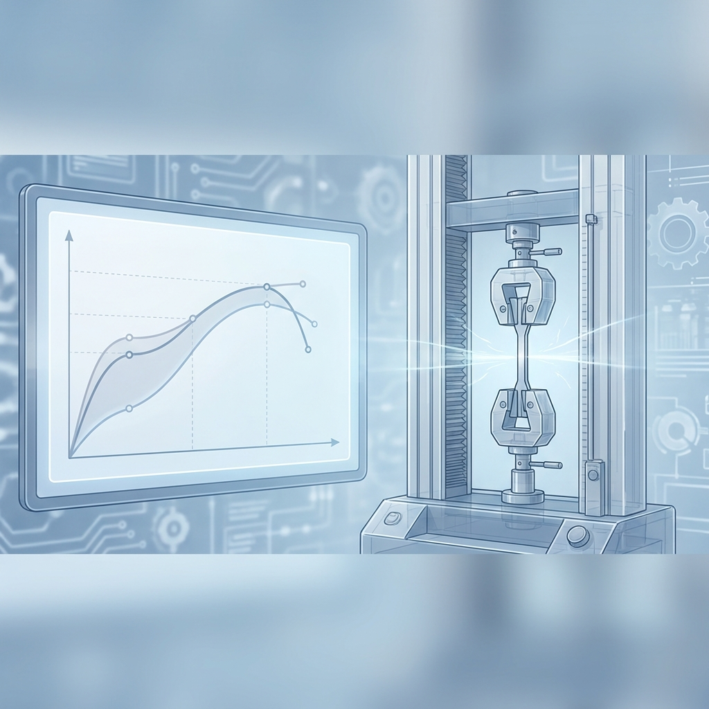
The Stress-Strain Curve Explained
The stress-strain curve is the most information-dense single graph in materials engineering. Generated by loading a standardized specimen to failure in a universal testing machine — following ASTM E8 for metals or ISO 6892-1 for international applications — it plots engineering stress against engineering strain at every instant of the test. Each point on the curve is a real measurement, taken as the specimen progresses from first loading to final fracture.
Reading a stress-strain curve correctly is a professional skill. The curve for a ductile metal like structural steel looks very different from the curve for a brittle ceramic or a compliant elastomer — and those differences encode everything an engineer needs to know about how a material will behave in service. Below is the complete sequence of events for a typical ductile metal:
| Stage | What Happens | Engineering Significance |
|---|---|---|
| 1 Elastic Region | Loading begins; stress and strain increase proportionally; Hooke’s Law applies; complete recovery on unloading | Slope = Young’s Modulus E; linear relationship |
| 2 Proportional Limit | End of perfectly linear stress-strain relationship; minor non-linearity may begin | Upper bound of strict Hooke’s Law applicability |
| 3 Elastic Limit | Maximum stress below which material still recovers fully; slightly above proportional limit in most metals | Last safe boundary before any permanent deformation |
| 4 Yield Point (Upper/Lower) | Stress at which plastic deformation begins; may show drop in steel (upper to lower yield point) | Critical design boundary; safety factors applied here |
| 5 Plastic Region (Strain Hardening) | Material deforms permanently; dislocations multiply and interact; stress continues to rise | Ductile materials absorb significant energy in this region |
| 6 Ultimate Tensile Strength (UTS) | Maximum stress the material can sustain; necking begins in ductile materials | Peak of the engineering stress-strain curve |
| 7 Fracture Point | Final failure; stress drops to zero; in ductile materials, significant reduction of area has occurred | End of test; used to calculate ductility and toughness |
The Elastic Region — Hooke’s Law in Action
In the elastic region, the stress-strain relationship is linear and fully reversible. Remove the load, and the material returns to exactly its original dimensions — the atomic bonds have been stretched but not permanently rearranged. This behavior is described by Hooke’s Law, formulated by Robert Hooke in 1678: σ = E × ε
The proportionality constant E is the Young’s Modulus (or Elastic Modulus), named after Thomas Young who formally defined it in 1807. Young’s Modulus represents the slope of the elastic portion of the stress-strain curve and is a direct measure of material stiffness. A steep slope indicates a stiff material (steel: E ≈ 200 GPa); a shallow slope indicates a compliant one (rubber: E ≈ 0.001–0.1 GPa).
Critically, Young’s Modulus is a material property — it is independent of specimen geometry. A steel rod and a steel plate will have the same modulus regardless of their cross-section or length. This is what makes it a universal design parameter: tabulated values from standard tests apply directly to any geometry made from the same alloy and heat treatment.
Practical application: A structural engineer designing a floor beam checks not only that stresses remain below yield strength, but that the deflection under service loads — calculated directly from Young’s Modulus — does not exceed allowable limits (typically L/360 for occupied floors per AISC standards).
Beyond Elasticity — Yield Point and Plastic Deformation
The yield point marks the most important boundary on the stress-strain curve from a structural design perspective. Below yield, the material behaves elastically and returns to its original form on unloading. Above yield, permanent plastic deformation occurs — atomic planes have shifted, and the original geometry cannot be recovered.
For many materials (particularly mild steel), the yield point is visible as a distinct peak on the curve, after which stress drops slightly and then continues at a lower level as plastic flow proceeds. For materials without a well-defined yield point (high-strength alloys, aluminum), the 0.2% offset method defines a practical yield strength: the stress at which a 0.2% permanent strain would remain on unloading.
After yielding, most ductile metals exhibit strain hardening: as dislocations multiply and interact, the material actually becomes stronger, requiring higher stress to continue deforming. This is why yield strength and ultimate tensile strength differ — and why cold-working processes (rolling, drawing, forging) increase the yield strength of metals.
Sequence from first loading to fracture in structural steel (ASTM A36):
- Elastic loading: stress increases linearly from 0 to approximately 250 MPa; full recovery on unloading.
- Upper yield point: brief stress peak at approximately 260 MPa; sudden atomic-level reorganization.
- Lower yield point: stress drops to approximately 250 MPa; plastic flow begins with little additional stress increase.
- Strain hardening: stress climbs steadily from 250 MPa toward ultimate tensile strength of 400–550 MPa.
- Ultimate tensile strength: peak stress; necking initiates at the weakest cross-section.
- Post-neck softening (engineering curve): apparent stress decreases as area at neck reduces dramatically.
- Ductile fracture: characteristic cup-and-cone fracture surface with significant elongation and reduction in area.
Plasticity is not always undesirable. In seismic design, engineers deliberately allow controlled plastic deformation in selected structural members during an earthquake — dissipating energy that would otherwise propagate as brittle fracture. This is why earthquake-resistant structures are designed with ductile detailing: managed plastic deformation is safer than sudden brittle failure.
Fracture Behavior — Ductile vs. Brittle Materials
The fundamental distinction between ductile and brittle fracture is visible immediately on the stress-strain curve: a ductile material shows substantial plastic deformation before fracture (large area under the curve beyond yield); a brittle material fractures with little or no plastic deformation (the curve ends near the elastic region).
| Ductile Material (e.g., Structural Steel) | Brittle Material (e.g., Cast Iron, Ceramics) |
|---|---|
| Significant plastic deformation before fracture | Fractures with minimal plastic deformation |
| Warning signs before failure: visible deformation, yielding | Sudden, without warning — no visible precursor deformation |
| High toughness (large area under curve) | Low toughness despite potentially high strength |
| Cup-and-cone fracture surface; rough texture | Flat, crystalline fracture surface |
| Failure mode predictable and manageable | Failure mode unpredictable; catastrophic potential |
| Preferred for structural applications with dynamic loads | Acceptable in compression-dominated, low-impact applications |
The safety implications are direct: ductile failure is preferable in most structural applications because it provides visible warning and energy absorption before final collapse. This principle drives material selection in earthquake engineering, impact-resistant packaging, and vehicle crash zone design — all applications where absorbing energy without sudden fracture is the design requirement.
Ready to Apply Stress-Strain Principles to Your Project? Get Expert Support Today
From material selection to failure analysis, our platform gives engineers access to expert resources, calculation tools, and guidance — practical support for real engineering challenges, available whenever you need it.
Access Engineering ToolsEngineering vs. True Stress-Strain
For most routine structural design, engineering stress-strain — calculated using original specimen dimensions throughout the test — is entirely adequate and is the industry standard. ASTM E8 and ISO 6892-1 both specify engineering measurements, and all tabulated material properties in design codes are engineering values. But for large-deformation analysis, the two approaches diverge significantly.
The critical difference appears after the yield point: as a specimen deforms, its cross-sectional area changes. Engineering stress uses the original area (A₀) throughout, meaning that after necking begins, the engineering curve shows decreasing stress. True stress uses the instantaneous area (A), revealing that — despite what the engineering curve suggests — the material is actually being stressed higher than ever at the moment of fracture.
| Engineering Stress-Strain | True Stress-Strain |
|---|---|
| σ_eng = F / A₀ (original area) | σ_true = F / A_instantaneous |
| ε_eng = ΔL / L₀ | ε_true = ln(L / L₀) (natural log) |
| Curve falls after UTS due to neck formation | Curve continues rising through fracture — true stress always increases |
| Standard for design codes, material databases | Required for large-deformation FEA, forming simulation, crash modeling |
| Simple to measure; requires only force and displacement | Requires real-time area measurement or indirect calculation from volume constancy |
Engineering Stress-Strain — The Practical Approach
Engineering stress-strain is calculated using the original cross-sectional area (A₀) and original gauge length (L₀) of the test specimen, measured before loading begins. The formulas are simply σ = F/A₀ and ε = (L − L₀)/L₀. This approach is standardized in ASTM E8/E8M (Metallic Materials, US) and ISO 6892-1 (International), ensuring that test results from different laboratories and different countries can be directly compared. For the vast majority of engineering design — where strains remain below 10–20% and geometric changes are small — engineering values are accurate enough and are mandated by design codes.
When engineering values are sufficient: Linear structural analysis, elastic design, standard material selection for beams, columns, and pressure vessels operating within design strain limits.
When they are not: Metal forming processes (deep drawing, extrusion), crash simulation, hyperelastic polymer analysis, or any application where strains routinely exceed ~10%.
True Stress-Strain — The Accurate Representation
True stress-strain accounts for the continuously changing geometry of a deforming specimen. After the onset of necking — the localized reduction in cross-section that occurs beyond ultimate tensile strength in ductile materials — the engineering and true curves diverge sharply.
For metals deforming below necking, conversion between engineering and true values is straightforward using volume-constancy (constant volume assumption): σ_true = σ_eng × (1 + ε_eng) and ε_true = ln(1 + ε_eng). After necking begins, direct measurement of instantaneous area is required — typically through optical or video extensometry.
In finite element analysis (FEA) for non-linear material behavior, true stress-strain curves are required as input to plasticity models (von Mises, Johnson-Cook). Using engineering values in a large-deformation FEA simulation introduces errors that increase dramatically with strain magnitude — a common source of inaccuracy in crashworthiness simulations run with improperly converted material data. SIMULIA (Abaqus) documentation covers non-linear plasticity material models in detail.
Material Properties Derived from Stress-Strain Analysis
The stress-strain curve is a compact representation of a material’s entire mechanical personality. Every major design parameter an engineer needs can be read directly from it — or calculated from it. The table below provides representative values for the materials most commonly encountered in structural and mechanical engineering (sourced from ASM Handbooks and MatWeb):
| Material | Young’s Modulus E (GPa) | Yield Strength (MPa) | UTS (MPa) | Elongation at Break (%) |
|---|---|---|---|---|
| Structural Steel (A36) | 200 | 250 | 400–550 | 20–23 |
| Aluminum Alloy (6061-T6) | 69 | 276 | 310 | 12–17 |
| Titanium Alloy (Ti-6Al-4V) | 114 | 880 | 950 | 14 |
| Concrete (compression) | 25–40 | N/A (compressive ~30 MPa) | ~3 (tensile) | ~0.01 |
| Natural Rubber | 0.001–0.1 | ~7 | ~30 | 400–800 |
| Carbon Fiber Composite | 70–200 | N/A | 600–3500 | 0.3–1.5 |
Understanding Moduli — Young’s, Shear, and Bulk
Young’s Modulus (E) is the most commonly used elastic modulus — it describes stiffness under uniaxial tensile or compressive loading and is the slope of the elastic region of the standard stress-strain curve. But it is one of three independent elastic moduli for isotropic materials:
| Modulus | Loading Condition | Governing Equation | Typical Application |
|---|---|---|---|
| Young’s Modulus (E) | Tensile or compressive axial loading | σ = E × ε | Beam deflection; column buckling; spring stiffness |
| Shear Modulus (G) | Shear loading; torsion | τ = G × γ | Shaft torsion; bolt shear; adhesive joint design |
| Bulk Modulus (K) | Uniform hydrostatic pressure | σ_vol = K × ε_vol | Deep-sea pressure vessels; hydrostatic loading of components |
A non-obvious but practically important observation: a material can have high stiffness under tension (high E) but significantly lower shear stiffness (G = E / 2(1+ν), typically 0.38–0.40 × E for metals). This means adhesive joints, bolted connections, and welded attachments — all primarily loaded in shear — must be designed using G, not E. Using Young’s Modulus for a shear-dominated calculation introduces a systematic overestimate of stiffness.
Strain Energy and Toughness — Materials Under Impact
The area under the stress-strain curve has direct physical significance: it represents the strain energy density absorbed by the material per unit volume as it deforms. This energy concept yields two important design parameters:
- Modulus of Resilience: Area under the elastic region only — the maximum elastic energy a material can absorb and release without permanent deformation. Calculated as σ_y² / (2E), where σ_y is yield strength. Relevant for springs, elastic connections, and any component designed to store and release energy elastically.
- Toughness: Total area under the complete stress-strain curve, from zero strain to fracture. Represents the total energy absorbed before failure. High-toughness materials (ductile steels, tough polymers) absorb more energy before fracturing than high-strength but brittle materials — which is precisely why toughness, not just strength, governs impact-resistance and crashworthiness design.
Practical example: two steels with identical yield strength can have dramatically different toughnesses if one has high ductility (large plastic region) and the other is more brittle (limited plastic deformation). For impact loading — a vehicle collision, a dropped load, a seismic event — the tougher steel is safer even if its yield strength is lower.
Real-World Applications of Stress-Strain Relationships
Stress-strain data is the currency of materials engineering across every industry that uses structural components. The specific properties extracted from the curve differ by application, but the analytical framework — apply force, measure stress and strain, characterize the curve — is universal.
| Industry | Application | Typical Material | Stress-Strain Data Used |
|---|---|---|---|
| Aerospace | Wing spar under aerodynamic fatigue loading | Titanium, aluminum alloys | Yield strength with large safety factor; fatigue life from cyclic S-N data |
| Civil/Structural | Bridge girder; high-rise column | Structural steel, concrete | Design to yield strength with safety factor per ASCE 7 / ACI 318 |
| Automotive | Crash zone energy absorption | High-strength steel, polymers | Toughness (area under curve); progressive plastic deformation |
| Biomedical | Orthopedic implant under walking loads | Ti-6Al-4V, CoCr alloys | Fatigue endurance; biocompatibility; Young’s modulus matching bone (~20 GPa) |
Designing with Stress-Strain Data
A systematic engineering design process using stress-strain data proceeds through several well-defined steps:
- Define the loading scenario: Identify all force types (tensile, compressive, shear, torsion), magnitudes, durations, frequencies, and environmental conditions (temperature, corrosion). This step determines which properties from the stress-strain curve will govern.
- Select candidate materials: Based on loading, identify candidates from materials databases (MatWeb, ASM Handbooks, material supplier datasheets). Compare Young’s Modulus, yield strength, and toughness against requirements.
- Apply design allowables: Structural codes (AISC for steel, ACI for concrete, ASME for pressure vessels) prescribe safety factors based on yield strength and ultimate tensile strength. Working stress = yield strength / safety factor. Safety factors typically range from 1.5 to 4.0 depending on consequence of failure and loading uncertainty.
- Check deformation limits: Even within elastic limits, deflections must be acceptable. Beam deflection depends directly on Young’s Modulus through δ = FL³ / (48EI) for a mid-span loaded beam. If deflection exceeds allowable limits, either material stiffness must increase or cross-section must be larger.
- Verify with analysis or test: Complex geometries require FEA to verify stress distributions. Critical applications require physical testing of representative specimens or full-scale prototypes. Test results are validated against the material’s stress-strain curve.
Case Studies — Success and Failure Analysis
Two instructive cases illustrate how stress-strain understanding — or its absence — determines structural outcomes.
Success: Seismic Retrofit
A 1960s steel frame building required seismic retrofit. The original steel (A7, yield strength 220 MPa) was found through testing to have adequate strength but insufficient ductility — the stress-strain curve showed limited plastic deformation before fracture. Rather than replacing all structural members, engineers added ductile steel link beams in the lateral force system, providing the energy-absorbing plastic deformation required by current seismic codes. The retrofit decision was directly driven by comparison of stress-strain curves for original and retrofit material.
Failure: Aluminum Temper Mismatch
A fabricated aluminum structure for an automated manufacturing system failed prematurely in service. Investigation revealed that the design used Young’s Modulus for 6061-T6 aluminum (69 GPa) for deflection calculations but actually procured 6061-T0 (annealed) material (Young’s Modulus similar but yield strength reduced from 276 MPa to approximately 55 MPa). Yield was being exceeded at normal operating loads — causing progressive permanent deformation that misaligned the system. The stress-strain curves for both temper states were visually and quantitatively different; material specification and incoming inspection procedures were subsequently strengthened.
Tensile Testing — How Material Properties Are Measured
The stress-strain curve is not an abstraction — it is generated through a physical test conducted on a standardized specimen in a universal testing machine (UTM). The standard procedure follows ASTM E8/E8M for metallic materials (US) or ISO 6892-1 (international).
The test specimen — typically a dog-bone shape with reduced cross-section in the gauge region — is gripped at each end by hydraulic or mechanical grips. Load is applied at a controlled rate (displacement-controlled is preferred for capturing post-yield behavior). Deformation in the gauge section is measured by an extensometer or strain gauge bonded to the specimen surface.
Standard tensile test procedure:
- Mount specimen in testing machine; zero force and displacement readings.
- Attach extensometer to gauge section; record gauge length L₀.
- Begin loading at specified displacement rate (ASTM E8: 0.005/min in elastic region).
- Record force (F) and extension (ΔL) continuously; software calculates stress and strain in real time.
- Continue loading through yield, strain hardening, UTS, necking, and fracture.
- Remove specimen; measure final gauge length and minimum cross-section for elongation and reduction-of-area calculations.
Every point on the stress-strain curve corresponds to a specific moment in this test — a real force measurement at a real time. The curve is not interpolated or inferred; it is directly measured. This is what makes it the authoritative source of mechanical property data for engineering design.
Advanced Concepts in Stress-Strain Analysis
The linear elastic model — Hooke’s Law, constant Young’s Modulus, fully reversible deformation — is an idealization that describes the behavior of metals at moderate loads and temperatures with useful accuracy. Real materials are more complex, and several important engineering contexts require moving beyond this simplified model.
Beyond Linear Elasticity — When Advanced Models Are Required
- Polymers and elastomers: highly non-linear stress-strain behavior; significant time-dependence (viscoelasticity).
- High-temperature metallic components: creep (time-dependent deformation at constant stress) becomes significant above 0.3–0.5 × melting temperature.
- High-strain-rate loading (impact, blast): dynamic Young’s Modulus and yield strength differ from quasi-static values by factors of 2–10.
- Cyclic loading (fatigue): stress-strain behavior under repeated load cycles differs from monotonic behavior; hysteresis loops and progressive ratcheting.
- Large deformations: engineering and true stress-strain diverge; geometric non-linearity must be accounted for in FEA.
Non-Linear and Time-Dependent Behavior
Many engineering materials — all polymers, biological tissues, some metals at elevated temperature — do not follow Hooke’s Law even at modest stresses. Their stress-strain relationship is non-linear from the very beginning of loading, and their response depends on both the magnitude of loading and its duration or rate.
- Viscoelasticity: Stress depends on both strain and strain rate. A polymer dashpot under a sudden constant strain shows stress that relaxes over time (stress relaxation). Under constant stress, it continues to deform (creep). Neither behavior is captured by a static stress-strain curve; a family of time-dependent curves is required.
- Creep: Time-dependent plastic deformation under sustained stress below yield strength, most significant at elevated temperatures. Turbine blades, boiler tubes, and reactor components are designed specifically against creep failure using stress-rupture and creep rate data.
- Strain-rate sensitivity: At impact speeds (bullet, explosion, vehicle collision), metals resist deformation at significantly higher stress levels than under slow loading. The Johnson-Cook material model captures this rate-dependence and is widely used in crash simulation.
Engineers working with polymers, composites, or elevated-temperature applications must treat standard (quasi-static, room-temperature) stress-strain data as a starting point, not a complete description.
Modern Testing and Measurement Techniques
Mechanical testing has evolved substantially since the first tensile machines of the early 20th century. The underlying stress-strain principles remain identical; the measurement methods have become dramatically more precise and informative.
- Digital Image Correlation (DIC): A full-field, non-contact optical strain measurement technique. A random speckle pattern applied to the specimen surface is tracked by high-resolution cameras as the specimen deforms. Software computes strain at every point on the surface — revealing heterogeneous strain distributions, crack initiation sites, and 3D deformation that a single-point extensometer cannot capture.
- Nanoindentation: Applies a precisely controlled load through a diamond tip at nanometer scales, generating a local load-displacement curve from which elastic modulus and hardness can be calculated at microscopic resolution. Essential for thin films, coatings, and biological materials.
- FEA validation: Experimental stress-strain data from physical tests is used to validate finite element models — and conversely, FEA predictions guide experimental design. The two approaches are complementary: experiments provide material properties; FEA extends those properties to complex geometries and loading conditions that cannot be tested directly. ScienceDirect hosts peer-reviewed research on these methods.
These technologies improve measurement fidelity, but they do not change the fundamental stress-strain relationship. A more accurate measurement of the curve is still a measurement of the same curve that Hooke described in 1678 and Young quantified in 1807.
Ready to Put Stress-Strain Knowledge to Work? Start Here
From material databases and design calculators to expert consultations and testing resources — our platform gives engineers everything needed to apply stress-strain principles with confidence in real projects.
Start Using Engineering ToolsConclusion — The Ongoing Importance of Stress-Strain Understanding
Materials science and computational power have together transformed engineering practice: finite element software can model geometrically complex structures under dynamic loading in hours, not months. But every one of those simulations depends on accurate material models — and every material model ultimately derives from stress-strain data measured in a laboratory. The more powerful the computational tool, the more important it is to understand the physical meaning of the data that feeds it.
Engineers who deeply understand the stress-strain curve — who can look at it and immediately identify yield strength, ductility, toughness, and elastic modulus, and reason about what each means for their design — make better material selection decisions, catch modeling errors before they propagate, and communicate more effectively with testing labs, material suppliers, and review bodies. A deep understanding of materials science — beginning with the stress-strain curve — remains the foundation for every engineering decision involving material behavior.
5 Key Principles to Take Forward
- Stress (σ = F/A) is internal resistance per unit area; strain (ε = ΔL/L₀) is dimensionless deformation. Stress causes strain.
- The elastic region obeys Hooke’s Law (σ = E × ε); Young’s Modulus is the slope and measures stiffness. Below yield, deformation is fully recoverable.
- The yield point is the critical design boundary. Working stresses must be kept below yield strength multiplied by the applicable safety factor.
- Ductile failure (with warning) is safer than brittle failure (without warning). Toughness — area under the entire curve — governs impact and energy-absorption design.
- Engineering stress-strain is sufficient for most design tasks. True stress-strain is required for large-deformation simulation, metal forming, and crash analysis.
References
- 1.Beer, F., Johnston, E., & DeWolf, J.. Mechanics of Materials (2020)
- 2.Callister, W. & Rethwisch, D.. Materials Science and Engineering: An Introduction (2020)
- 3.Hibbeler, R.. Mechanics of Materials (2022)
- 4.ASTM E8/E8M. Standard Test Methods for Tension Testing of Metallic Materials (2022)
- 5.ISO 6892-1. Metallic Materials — Tensile Testing at Room Temperature (2019)
- 6.NIST. Material Measurement Laboratory — Physical measurement standards and calibration (2025)
- 7.ASM International. Handbook of Materials Properties (ASM Handbooks) (2025)
- 8.MatWeb. Online Materials Information Resource (2025)
- 9.AISC. Steel Construction Manual (2022)
- 10.ACI 318. Building Code Requirements for Structural Concrete (2019)
- 11.ASME. Boiler and Pressure Vessel Code (2023)
- 12.SIMULIA (Abaqus). Non-linear plasticity material models documentation (2025)
- 13.International DIC Society. Digital Image Correlation guidelines (2025)
- 14.ScienceDirect. Peer-reviewed materials science research (2025)
Frequently Asked Questions

Written by
Valentina Lipskaya
Clinical Psychologist · Gestalt Therapist · CBT Specialist · ICF Certified Coach · MBA Professor
Panic Disorder, Anxiety, CBT & Gestalt Therapy
Valentina Lipskaya is a certified clinical psychologist and gestalt therapist specializing in panic disorders, anxiety, and neurological conditions. With over 15 years in psychology and 7 years of hands-on clinical practice, she has helped more than 750+ clients overcome panic, chronic anxiety, and psychosomatic conditions — without medication. Her work at Dzeny translates evidence-based therapeutic methods into practical, accessible guidance for everyday mental health.